Processing 2D, 3D and 4D Spectra with hmsIST
Assumed knowledge: NMRPipe, NMRDraw and the Unix Environment
In order for these tutorials to work you must have the program nmrPipe, nmrDraw and a C shell (csh or tcsh) installed on your linux or Mac OSX machine. Installation of nmrPipe and tutorials on how to work with this processing platform can be found on its website. Also a working knowledge of nmrDraw will be useful. Since nmrPipe runs under the C shell (csh or tcsh) environment, all examples below also assume you are running commands in csh or tcsh. Most linux distributions and the Mac OSX command line environment is the BASH shell by default. Please make sure you are in a C shell, not the BASH shell.
We will present examples of 2, 3 and 4D processing. We reccommend working through the 2D tutorial before diving into 3 and 4D as it is easier to understand and lays a good foundation for how things are done in higher dimensions. In fact, a ot of the details are skipped in the 3 and 4D tutorial as it's assumed you understand the 2D processing section.
Further examples (including example data) and presentations that we presented at ICMRBS_2014 can be found at:
https://www.dropbox.com/sh/axoufdmzi97da5y/AACZPWW1fpZGt2OJSa0DQeona?dl=0
For support with reconstructing NUS data with hmsIST, please join the forum by sending email to:
hmsist-subscribe@yahoogroups.com
Or by visiting:
https://groups.yahoo.com/neo/groups/hmsIST/info
Quick Links to:
2D Processing
3D Processing
4D Processing
Processing 2D Spectra
Once you have downloaded the example directory, unpack it with the following command
tar -zxvf HSQC.tar.gz
This will create a directory called 'HSQC' and contains a 1H-15N HSQC data set from a Bruker magnet. What applies here applies equally well to Varian/Agilent data sets.
Normally data sets are converted from Bruker (or Varian) data format to nmrPipe using a conversion script. The conversion script we will use is called fid.com. It's content are:
#!/bin/csh -f
#
bruk2pipe -in ser -DMX -swap -decim 24 -dspfvs 12   \
-xN              2048     -yN                80     \
-xT              1024     -yT                40     \
-xMODE            DQD     -yMODE  Echo-AntiEcho     \
-xSW         7002.801     -ySW         1824.568     \
-xOBS         500.130     -yOBS          50.678     \
-xCAR           4.697     -yCAR         118.000     \
-xLAB              1H     -yLAB             15N     \
-ndim               2     -aq2D          States     \
-out data.fid -ov -verb
This script takes the bruker 'ser' file and makes a data.fid file with appropriate frequency information and other labels. The command 'bruker' (or 'varian'), when entered as a command will generate this script for you (sometimes it gets information wrong, be advised). Note that the number of indirect complex points (-yT flag) seems somewhat truncated. This is because we only collected 40 complex points out of a total of 400 (10%). We will shortly fill in the missing data. First we will fourier transform the direct dimension (1H) and make sure it is phased correctly. We will use the nmrPipe script called 'ft1.com' to transform and we will check the result with nmrDraw. The ft1.com script is like a normal nmrPipe script except we only do a direct dimension transform:
nmrPipe -in data.fid                    \
| nmrPipe  -fn SOL                            \
| nmrPipe  -fn SP -off 0.3 -end 0.98 -pow 2   \
| nmrPipe  -fn ZF -auto                       \
| nmrPipe  -fn FT                             \
| nmrPipe  -fn PS -p0 0.0 -p1 0.0 -di         \
| nmrPipe  -fn EXT -left -sw -verb            \
| nmrPipe  -fn TP                             \
   -verb -ov -out test.nus
The data.fid file is read in, solvent suppresion (SOL), a window function (SP) is applied and we zero fill (ZF). We fourier trasform (FT) and then apply a phase correction (PS). Here we apply no phase correction (yet). We extract (EXT) the amide (left) side of the spectrum and finally we transpose the dimensions. The x (direct) dimension becomes y, and the y (indirect) becomes x, before writing out the file to test.nus. Lets take a look at this file in nmrDraw by issuing the following command
nmrDraw test.nus
The first thing you should notice is that despite the direct dimension beings the 'y' axis in the file, the direct, transformed dimension is still displayed in nmrDraw along the convention horizontal x-axis. It is however labeled 'Y'.
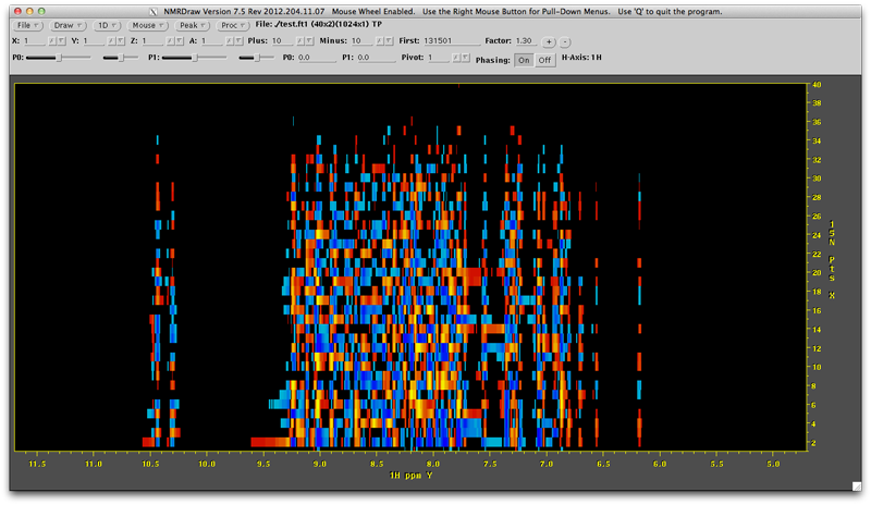
This may look odd because the vertical dimension is unprocessed. It is also just the samples that have been collected and so vertical lines through this data aren't even sinusoidal. Right mouse click the 'Mouse' menu and draw a 1D Horizontal line. The lines of blue and orange are distracting at this point so increase the contour level the with (+) button to the top right until you havea first contour level of around 4 million. Click the draw menu button. You will now see the horizontal 1D through the data. You need to phase this. The first indirect line (bottom of screen) is not ideal for this due to low signal intensity, but the second line from the bottom is not too bad. Click towards the bottom of the data until you have a line that looks like this (not the position of the purple line at the 15N point = 2 position):
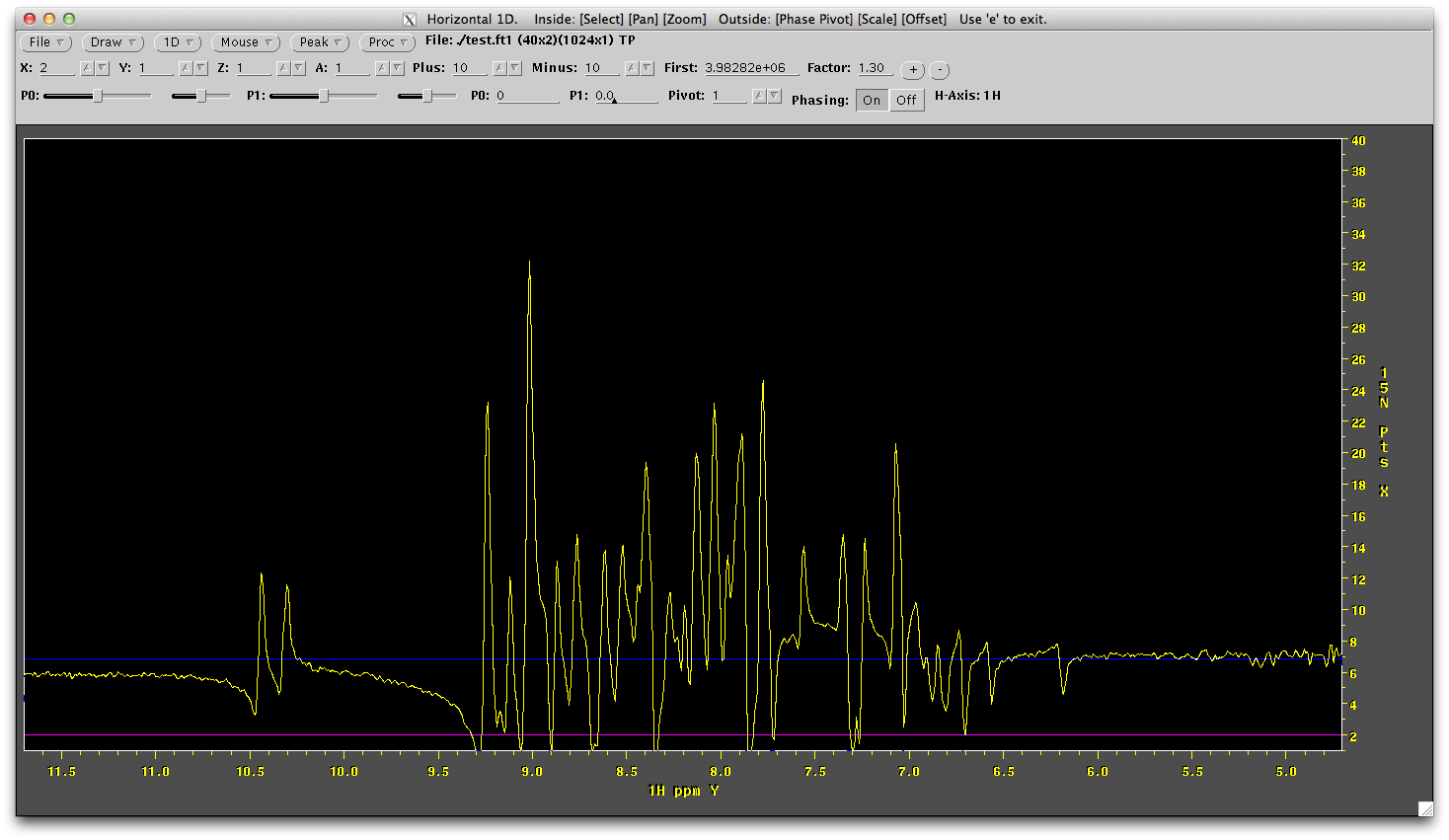
Use the P0 slider until it is phase, like below
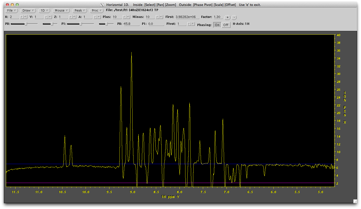
Not the phase correction required. In this case it is about +45.8. Lets apply this phase correction in the ft1.com file.. make sure the phasing line in the script now reads
| nmrPipe -fn PS -p0 45.8 -p1 0.0 -di \
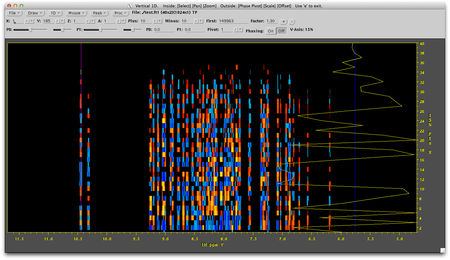
Rerun the script and again look at the result with
nmrDraw test.nus
If we also draw a vertical line through the streak of data most to the left (right click mouse, select 1D Vertical and click over the left most line of data) we will see that the vertical data is not a sinusoid.... yet.
It should look like this:
We will now reconstruct this dimension by using the schedule used to collect this data to fill in uncollected data as zeros (temporarily) and then reconstruct that data. To do this we will run a script that calls the istHMS software. This file is called 'ist' and looks like this:
#!/bin/csh

istHMS -ref 0 -vlist sched -xN 512 -itr 400 -user 1 -verb 0 \
< ./test.nus >! ./test.ft1
Here the istHMS program is run with several flag options. -vlist describes the schedule file. This file is called 'sched'. -xN denotes how many points total to reconstruct. If you look in the 'sched' file you will see we have points ranging from 0 to 399 (1st point to the 400th point). There is currently a bug in the program which means if we used an xN of 400 the reconstruction fails. Besides it makes sense to reconstruct to the next 'power of 2' number, s we will put 512 points here. This is 512 complex points. -itr is the number of iterations of reconstruction; we find 400 works well generally. The other flags are not important right now. We also direct in the test.ft1 file (< ./test.nus) and direct out the output of the reconstruction (>! ./test.ft1). I did say unix was assumed knowledge.
Running 'ist' does the reconstruction so long as you have a compatible linux machine and the istHMS software in that directory is able to run without a problem. If you have problems running istHMS in that directory, contact us. Alternatively, if you are on OSX, copy the file istHMSmac to istHMS and try running it. You may need to install the fftw3 libraries located here. Anyway, if it is running it will just sit there while its working, reporting nothing. If you need an output to see that it is working, change the ist script so the flag -verb now reads '-verb 1'. With this flag on you will get lots of incrementing numbers, showing you it is working.
This process produces a file called test.ft1. You can open it with nmrDraw
nmrDraw test.ft1
Like before, only one dimension is transformed but now sinusoidal data has been reconstructed in the indirect dimension. The number of points now is also 512. Like above, draw a 1D vertical along the left most line of data and you will see its a nice signal, just waiting to be Fourier transformed.
This is now ready to be transformed in the indirect dimension. We turn to nmrPipe to do this and use the script called ft2.com
nmrPipe -in test.ft1 \
| nmrPipe  -fn SP -off 0.3 -end 0.98 -pow 1 -size 512  -c 0.5   \
| nmrPipe  -fn ZF -size 1024                                    \
| nmrPipe  -fn FT                                               \
| nmrPipe  -fn PS -p0 90.0 -p1 0.0 -di                          \
| nmrPipe  -fn POLY -ord 0 -auto                                \
| nmrPipe  -fn TP                                               \
| nmrPipe  -fn POLY -ord 0 -auto                                \
   -verb -ov -out test.ft2
This reads in the file test.ft1. Recall that the indirect dimension is in the x dimension as far as nmrPipe is concerned so when we apply functions they are being applied along the indirect dimension. We first apply an SP window function, zero fill to 1024 points (usual practice for 512 complex points) and we FT. The phase correction here is 90.0. If it is off, you can always phase it like we did above but in the vertical direction. We apply a POLY base line correction, transpose so the direction dimension is now 'x' again and then again apply a POLY base line correction in this dimension. Finally we write out the file to 'test.ft2'. See the results by running:
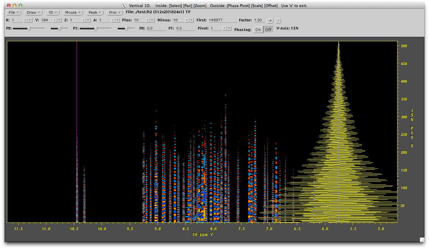
nmrDraw test.ft2
Looks awesome! And collected in 1/10th of the time.
We can simplify this processing by combining all these steps into one script. It has the disadvantage that it completes reconstruction before you know you have phased your direct dimension correctly. Incorrect phasing in the first dimension impacts reconstruction minorly, but it can be harder to get correct phase information from a reconstructed spectrum incorrectly phased. Plus reconstruction takes significantly more time - it is nice to only have to do it once.
Despite all that, here is a script that will perform the entire process for you. It is called ft12.com in the sample directory:
nmrPipe -in data.fid                            \
| nmrPipe -fn SOL                                     \
| nmrPipe -fn SP -off 0.3 -end 0.98 -size 512 -c 1.0  \
| nmrPipe -fn ZF -auto                                \
| nmrPipe -fn FT -auto                                \
| nmrPipe -fn PS -p0 45.8 -p1 0.0 -di                 \
| nmrPipe -fn EXT -left -sw -verb                     \
| nmrPipe -fn TP                                      \
| istHMS -xN 512 -sched ./sched -itr 400              \
| nmrPipe -fn SP -off 0.5 -end 0.98 -c 0.5  -size 512 \
| nmrPipe -fn ZF -auto                                \
| nmrPipe -fn FT -auto                                \
| nmrPipe -fn PS -p0 -90.0 -p1 0.0 -di -verb          \
| nmrPipe -fn POLY -ord 0 -auto                       \
| nmrPipe -fn TP                                      \
| nmrPipe -fn POLY -ord 0 -auto                       \
        -ov -out test.ft2
Processing 3D Spectra
Processing of a 3D (and 4D) spectrum is conceptually a little different from the 2D case. This is because data is no longer collected in planes. For example, a triple resonance 3D set may be collected as a series of 1H-15N planes with increasing 13C evolution and data is stored in this order. Because we collect data as a limited set of preselected points, data is simply stored in the order of the points in the schedule file.
Each point in a 3D set is made up of 4 FIDs. The actual FIDs contain direct (1H) time domain data that can be transformed directly; this direct dimension time domain data is not acquired non-uniformly. The reason there are 4 FIDs for each point is because each indirect dimension (2 in this case) must have 2 series of data to compose a complex point. Often the 15N dimension has complex data acquired by collecting an echo/antiecho pair while the 13C dimension is acquired by states-TPPI. In both cases 2 series of data are required. Thus, for each point of data collection, there are 4 FIDs. For a 4D data set there are 8 FIDs for each point (se processing 4D spectra).
Lets start to see this in action by untaring the example data set
tar -zxvf HNCO.tar.gz
In the HNCO directory that is created you will see a file called fid.com which converts the data from the spectrometer into nmrpipe format. It looks like this
#!/bin/csh

bruk2pipe -in ./ser \
  -bad 0.0 -noaswap -DMX -decim 24 -dspfvs 12 -grpdly 0  \
  -xN              2048  -yN                 4  -zN               818  \
  -xT              1024  -yT                 2  -zT               409  \
  -xMODE            DQD  -yMODE           real  -zMODE           real  \
  -xSW         7002.801  -ySW         1824.818  -zSW         2777.778  \
  -xOBS         500.132  -yOBS          50.684  -zOBS         125.780  \
  -xCAR           4.772  -yCAR         119.571  -zCAR         176.054  \
  -xLAB              HN  -yLAB             15N  -zLAB             13C  \
  -ndim               3  -aq2D          States                         \
| nmrPipe -fn MAC -macro $NMRTXT/ranceY.M -noRd -noWr   \
| pipe2xyz -x -out ./fid/test%03d.fid -verb -ov -to 0
This convert file can be also generated from the directory by using the nmrpipe programs 'bruker' or 'varian'. They may however make some mistakes. The important things to note is that the 'y' dimension has only 4 points in it. This is because of the reasons described above. The 'z' dimension has the number of points collected in it (our example is 818 points out of 8192 points, or 10%). Here the mode of collection has been set to 'real' because at this stage we want each FID to be treated individually and not as complex pairs. We do however need to label the 'y' dimension as Echo-Antiecho (or as Rance-Kay) data collection mode (this of course depends on your pulse sequence). We do this with the line:
| nmrPipe -fn MAC -macro $NMRTXT/ranceY.M -noRd -noWr \
We then save the data as a series of 'fid' files in the fid directory. Run:
fid.com
and you will see there are 818 files in the fid directory. We can look at these files in nmrDraw but they are not very interesting. First, lets do a fourier transform on all these FIDs so we can look at the data with the direct dimension in the frequency domain. Execute the following command:
ft1xyz.com
This script looks like this:
#!/bin/csh -f

rm -rf xyz

xyz2pipe -in fid/test%03d.fid -x \
| nmrPipe -fn SOL \
| nmrPipe  -fn SP -off 0.3 -end 0.98 -pow 2 -c 0.5  \
| nmrPipe  -fn ZF -auto                          \
| nmrPipe  -fn FT -verb                             \
| nmrPipe  -fn PS -p0 0.0  -p1 0.0 -di              \
| nmrPipe  -fn EXT -left -sw           \
| pipe2xyz -ov -out xyz/test%03d.nus -x
The reason why we have xyz appended to the name is because the output of this script preserves the order of the data in the nmrPipe files (x=1H, y=15N, z=13C). Later we change this order, but for now we need it in this order so we can phase correct our data. After running ft1xyz.com lets look at the data in nmrDraw. OUr files are in the xyz directory and end in the file name '.nus'.
nmrDraw xyz/test001.nus
This shows us the first 4 FIDs for the first indirect point (this point should always be 0,0 - always collected a 0,0 point - no excuses). The setup of this pulse sequence means we have full signal in the first FID (first 15N point), no signal in the second FID (second 15N point) and no signal in the next two FIDs (the complex points of the 13C dimension). In total we should only see significant signal in the first (bottom) FID. Right click on the 'mouse' menu and draw a 1D horizontal line. Click near the bottom to draw the line over the first FID. You will see something like this below. Note it is not phased.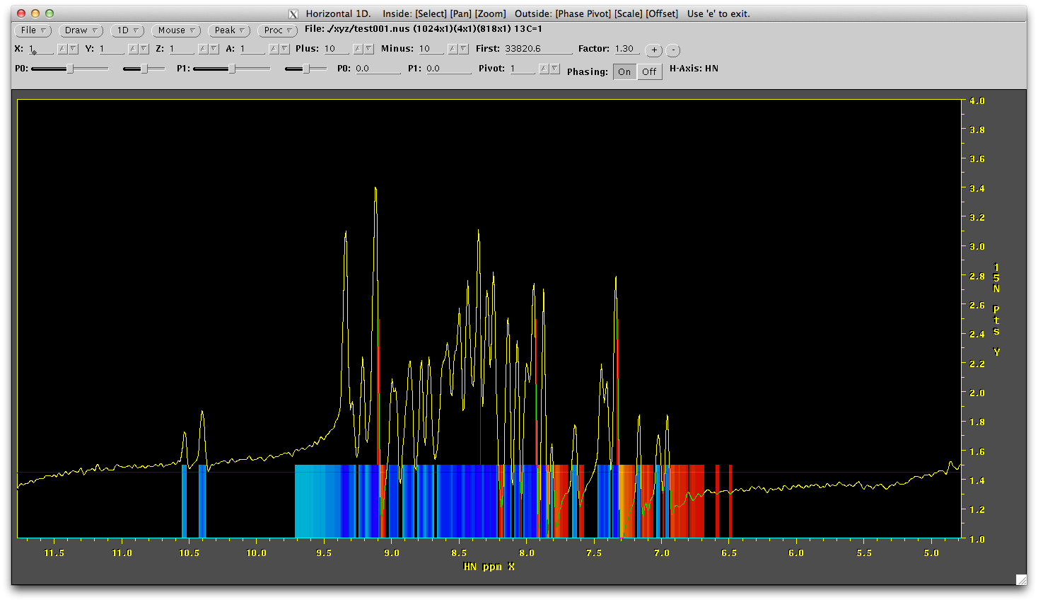
Lets phase correct it as above in the 2D example and apply the phase correction in the ft1xyz.com file and rerun it. Change the PS line in ft1xyz.com to this:
| nmrPipe -fn PS -p0 -28.2 -p1 0.0 -di \
Then run
ft1xyz.com
And now lets look at the data again:
nmrDraw xyz/test001.nus
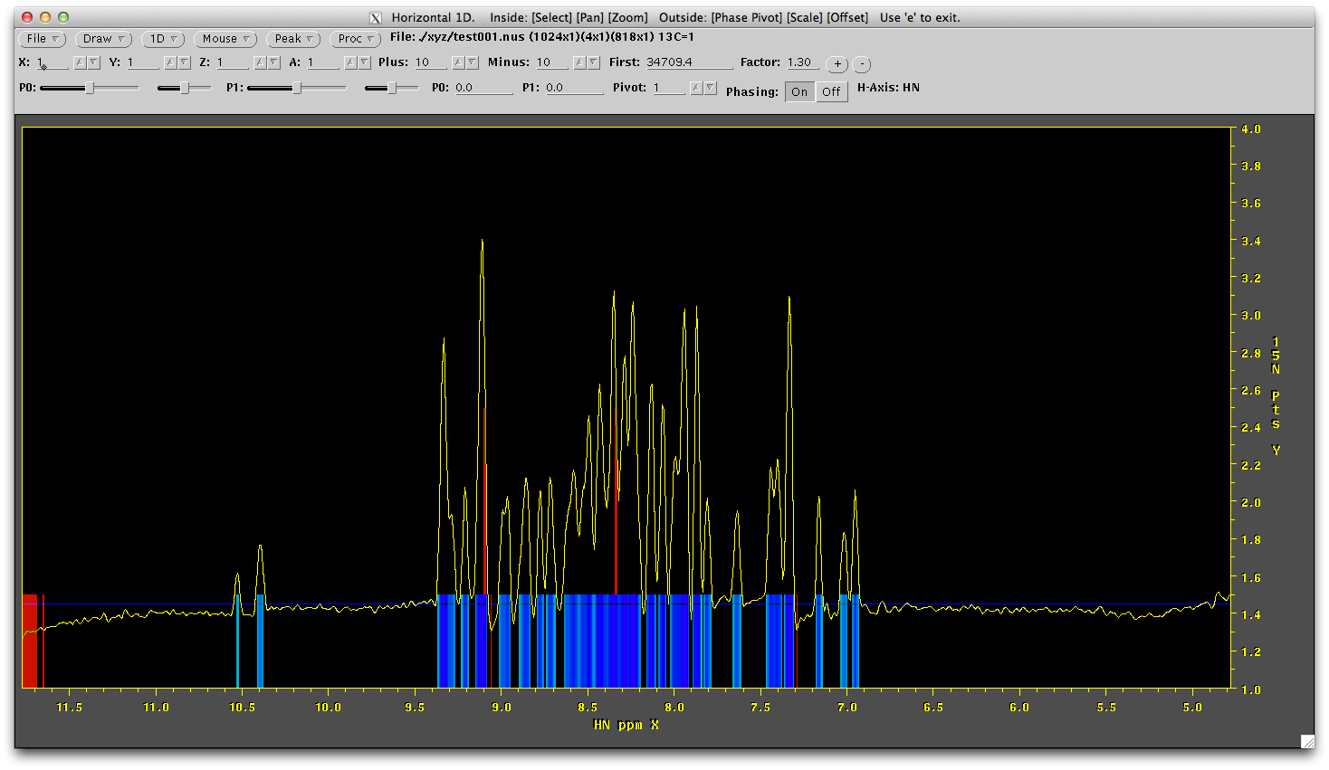
Now all 818 points should be phase corrected in the direct dimension. Before we can do reconstruction of the missing data we need to change the order of the data so the 15N and 13C dimensions are 'first' and 'second' in the file. This is acheived easily by changing the way the data is written out after transformation. The script 'ft1.com' is set up to do this. However, we need to make sure we phase the direct dimension correctly again, so edit ft1.com and correct the PS information and run this script. It should look something like this:
#!/bin/csh -f

rm -rf yzx # clean up
rm -rf yzx_ist # clean up
mkdir yzx
mkdir yzx_ist

xyz2pipe -in fid/test%03d.fid -x \
| nmrPipe -fn SOL \
| nmrPipe  -fn SP -off 0.3 -end 0.98 -pow 2 -c 0.5 \
| nmrPipe  -fn ZF -auto                          \
| nmrPipe  -fn FT -verb                             \
| nmrPipe  -fn PS -p0 -28.2 -p1 0.0 -di              \
| nmrPipe  -fn EXT -left -sw           \
| nmrPipe  -fn POLY -auto -ord 1 \
| pipe2xyz -ov -out yzx/test%03d.nus -z
Now we are ready to do reconstruction of the missing data.
Reconstruction is computationally expensive but not excessively so. It can be performed in resonable time (< 1 hr) on most modern cpus and even faster on a cluster. We provide two ways in which to do reconstruction. 1) Local, meaning on your desktop or laptop and 2) On a cluster. Simple scripts for doing these are provided in the sample directory and are called
run.local
and
run.cluster
run.local is simple but does rely on another program to exploit all available cpus and threads on your machine (or a subset if you wish). This program is called 'parallel' and additional details can be found here. The 'parallel' program has been included in the sample files. run.local looks like this:
parallel -j 100% './ist.csh {} > /dev/null; echo {}' ::: yzx/test*.nus
The -j option allows you to nominate how much of the available cpu resources to devote to the process. I've set it to 100% which works on my macbook pro just fine. The command that is actually executed is ist.csh (see below) - it takes arguments that are symbolically replaced with '{}' for now. We also 'echo' the contents of '{}'. When interpreted, the '{}' is replaced with the files selected with 'yzx/test*.nus' - that is all the files in the yzx directory. In effect the program 'parallel' will one by one execute ist.csh with each file in the yzx directory, however it will lauch as many processes as possible allowed by the '-j' flag.
The ist.csh command is a simple script as can be seen below
#!/bin/csh

set F = $1

set in = $F:t
set out = $F:t:r.phf


echo $in $out

istHMS -dim 2 -incr 1 -xN 64 -yN 128 -user 1  \
    -itr 400 -verb 0 -ref 0 -vlist ./sched.2d \
    < ./yzx/${in} >! ./yzx_ist/${out}
The contents of this script allow istHMS to reconstruct each 15N/13C plane and has similar options to 2D reconstruction above. A full list of the command line options for istHMS is forthcoming. This process takes some time to execute on a laptop or desktop. My macbook pro does this process in about 25 minutes. There are two ways to make this process shorter. Firstly, you can trim the direct dimension as much as pssible in ft1.com. Secondly you can adjust the number of iterations (400 here) however with decreasing number of iterations, quality of the reconstruction degrades. For this to work on a mac you will have to copy istHMSmac to istHMS first.
Reconstructions can also be done on a cluster. We have an example run.cluster file that runs the process on our cluster. Since cluster architectures vary we leave it up to you and your sys-admin to make this work.
Once the reconstruction has finished, the format of the data is still in a 'linear' or 'phase first' order. That is, it is not arrayed into planes. The next step changes this order into plane order (conventional nmrPipe format). We do this with the script phf2pipe.com which executes a program called phf2pipe. If on a mac, copy phf2pipemac to phf2pipe first. Then run:
phf2pipe.com
This reorders the data into planes and now can be conventionally transformed by nmrPipe. The output is put into a directory called 'rec'. An example script to do this is ft23.com:
#!/bin/csh -f

#
# 3D States-Mode HN-Detected Processing.

xyz2pipe -in rec/test%03d.ft1 -x \
| nmrPipe  -fn SP -off 0.5 -end 0.98 -pow 2 -c 0.5 \
| nmrPipe  -fn ZF -auto                       \
| nmrPipe  -fn FT -verb                           \
| nmrPipe  -fn PS -p0 0.0 -p1 0.0 -di              \
| nmrPipe -fn REV -verb \
| nmrPipe  -fn TP \
| nmrPipe  -fn SP -off 0.5 -end 0.98 -pow 2 -c 0.5 \
| nmrPipe  -fn ZF -auto  \
| nmrPipe  -fn FT -di  -alt -verb                       \
#| nmrPipe  -fn PS -p0 -90.0  -p1 180.0 -di              \
#| nmrPipe  -fn TP \
#| nmrPipe  -fn ZTP \
> rec/data.pipe
pipe2xyz -in rec/data.pipe -out rec/test%03d.ft3 -x
This inputs the files from the rec directory (ending in ft1 - they are transformed in 1 dimension only) and transforms in the reimaining 2 dimensions. First diemsion that is read in is the 15N dimension in this example. There is no need for a phase correction here, however the dimension needs to be reversed. We then transpose and make 13C the active dimension and FT again. An -alt flag is needed this time. No phase correction is required. I have also commente dout a number of final transpositions that may order the data in ways you prefer. Finally data is output to rec/data.pipe and then converted to xyz format for viewing in nmrDraw. So run ft23.com:
ft23.com
and lets look at one of the 15N/13C planes with:
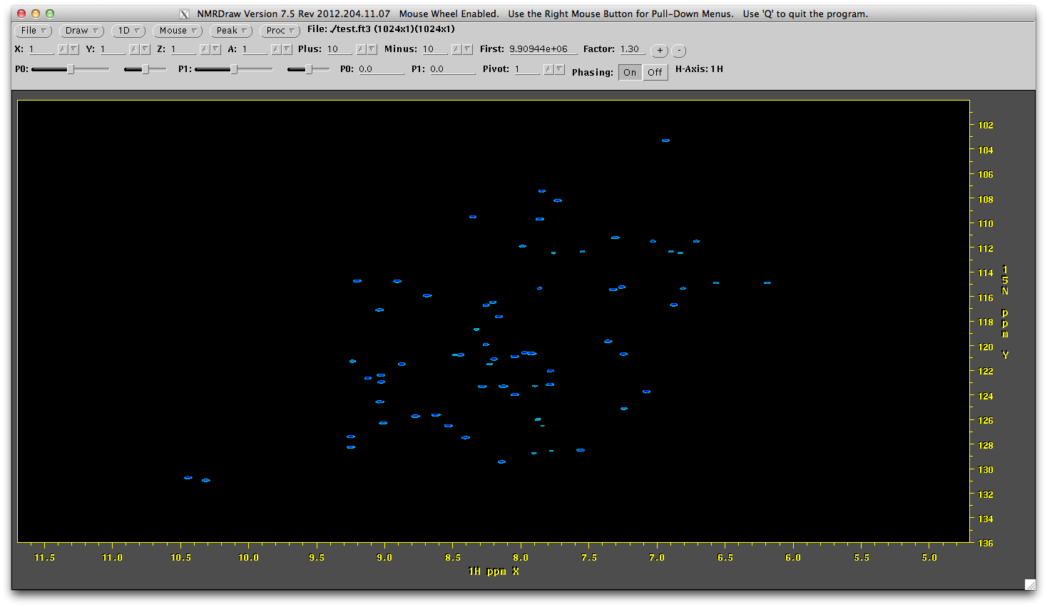
nmrDraw rec/test315.ft3
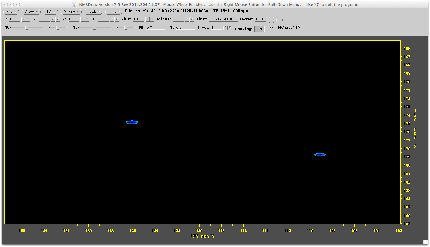
You can see the reconstruction has worked. You can look at the entire sprectrum by launching nmrDraw and viewing all the files in the rec directory (ending in ft3).
Please note that the current example HNCO has some artifacts that are the result of collecting this spectrum under xwinnmr (we don't recommend it). They can be seen in the 15N dimension - these do not occur when running good sequences under topspin 2.1 and higher.
Processing 4D Spectra
Coming...
